使用Python从头开始构建一个百万参数的LLM
逐步指南:复制LLaMA架构

制作自己的大型语言模型(LLM)是一件很酷的事情,许多像谷歌、推特和脸书这样的大公司都在进行这项工作。它们发布不同版本的模型,如70亿、130亿或700亿。甚至较小的社区也在进行这样的工作。你可能已经阅读过关于制作自己的LLM的博客或观看了相关视频,但它们通常更多地谈论理论,而不是实际的步骤和代码。
在这篇博客中,我将尝试制作一个仅包含230万个参数的LLM模型,有趣的是我们不需要花哨的GPU。我们将遵循LLaMA 1论文的方法来引导我们。不用担心,我们会保持简单,并使用一个基本数据集,以便您能够看到创建自己的百万参数LLM模型是多么容易。
请查看我的新博客,我通过矩阵乘法手工解析了变形金刚架构。我逐步分解,让你轻松掌握概念。
目录
· 先决条件· 理解LLaMA的Transformer架构 ∘ 使用RMSNorm进行预归一化 ∘ SwiGLU激活函数 ∘ 旋转嵌入(RoPE)· 设定舞台· 数据预处理· 评估策略· 设置基本神经网络模型· 复制LLaMA架构 ∘ RMSNorm进行预归一化 ∘ 旋转嵌入 ∘ SwiGLU激活函数· 尝试超参数 ·保存您的语言模型(LLM)· 结论
前提条件
确保您对面向对象编程(OOP)和神经网络(NN)有基本了解。熟悉PyTorch在编码过程中也会有所帮助。
理解LLaMA的Transformer架构
在深入创建我们自己的LLM(Long Language Model)之前,使用LLaMA方法,了解LLaMA架构是至关重要的。下面是香草变压器(vanilla transformer)和LLaMA之间的比较图表。
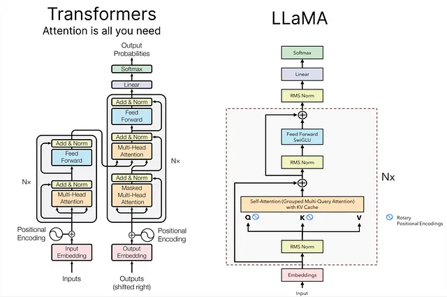
如果您对香草变压器架构不熟悉,您可以阅读此博客了解基本指南。
让我们更详细地了解LLaMA的基本概念:
使用RMSNorm进行预处理:
在LLaMA方法中,采用一种称为RMSNorm的技术来对每个变压器子层的输入进行归一化。这种方法受到GPT-3的启发,旨在优化与层归一化相关的计算成本。RMSNorm能够提供与层归一化相似的性能,但显著减少运行时间(约7%∼64%)。
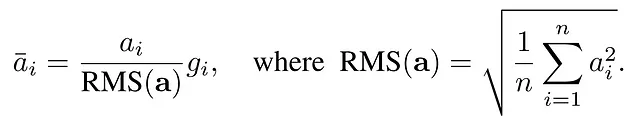
它通过强调重新缩放不变性并根据均方根(RMS)统计量调整总和输入来实现此目标。主要动机是通过删除均值统计量来简化层归一化。有兴趣的读者可以在此处探索RMSNorm的详细实现。
SwiGLU 激活函数:
LLaMA引入了SwiGLU激活函数,其灵感来源于PaLM。要理解SwiGLU,首先要掌握Swish激活函数是至关重要的。SwiGLU扩展了Swish,并涉及一个自定义层,其中包含一个密集网络来分割和乘以输入激活。
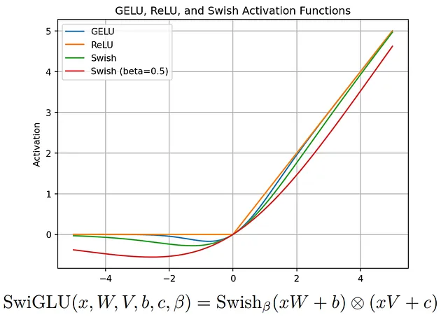
目标是通过引入更复杂的激活函数来增强模型的表达能力。有关SwiGLU的更多详细信息,请参阅关联论文。
旋转嵌入(RoPE):
旋转嵌入,也称为RoPE,是在LLaMA中使用的一种位置嵌入类型。它利用旋转矩阵编码绝对位置信息,并在自注意力公式中自然地包含显式相对位置依赖。RoPE具有可适应各种序列长度和随相对距离增加而衰减的单词间依赖性等优势。
这是通过使用旋转矩阵对相对位置进行乘法编码来实现的,从而导致相对距离的衰减 — 这是自然语言编码中的一个可取特性。对数学细节感兴趣的人可以参考RoPE论文。
除了这些概念,LLaMA论文还介绍了其他重要的方法,包括使用具体参数的AdamW优化器,高效的实现,如在xformers库中可用的因果多头注意力操作符,以及手动实现的反向函数,以优化反向传播过程中的计算。
一个特别的致谢和感谢给Anush Kumar,为LLaMA的每个关键方面提供了详尽的解释。
设定舞台
我们在整个项目中将使用多种Python库,因此让我们将它们导入:
# PyTorch for implementing LLM (No GPU)
import torch

# Neural network modules and functions from PyTorch
from torch import nn
from torch.nn import functional as F

# NumPy for numerical operations
import numpy as np

# Matplotlib for plotting Loss etc.
from matplotlib import pyplot as plt

# Time module for tracking execution time
import time

# Pandas for data manipulation and analysis
import pandas as pd

# urllib for handling URL requests (Downloading Dataset)
import urllib.request
此外,我正在创建一个配置对象,用于存储模型参数。
# Configuration object for model parameters
MASTER_CONFIG = {
    # Adding parameters later
}
这种方法保持了灵活性,使得将来可以根据需要添加更多的参数。
数据预处理
在原始的LLaMA论文中,使用了多样的开源数据集来训练和评估模型。
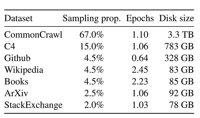
不幸的是,对于较小的项目来说,利用大规模数据集可能并不实际。因此,对于我们的实现,我们将采取一种更为谦逊的方法,通过创建一个大幅缩减的LLaMA版本。
考虑到没有访问大量数据的限制,我们将专注于使用TinyShakespeare数据集训练一个简化版本的LLaMA。这个开源数据集可以在这里找到,包含了大约40,000行来自莎士比亚作品的文本。这个选择受到了Karpathy的Makemore系列的影响,该系列提供了训练语言模型的宝贵见解。
虽然LLaMA是基于一个包含1.4万亿标记的广泛数据集进行训练的,但是我们的数据集TinyShakespeare仅包含约100万个字符。
首先,让我们通过下载来获取我们的数据集:
# The URL of the raw text file on GitHub
url = "https://raw.githubusercontent.com/karpathy/char-rnn/master/data/tinyshakespeare/input.txt"

# The file name for local storage
file_name = "tinyshakespeare.txt"

# Execute the download
urllib.request.urlretrieve(url, file_name)
这个Python脚本从指定的URL获取tinyshakespeare数据集,并以文件名“tinyshakespeare.txt”保存在本地。
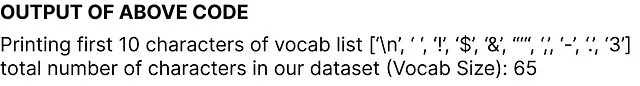
接下来,让我们确定词汇量,它代表着我们数据集中独特字符的数量。下面是代码片段:
# Read the content of the dataset
lines = open("tinyshakespeare.txt", 'r').read()

# Create a sorted list of unique characters in the dataset
vocab = sorted(list(set(lines)))

# Display the first 10 characters in the vocabulary list
print('Printing the first 10 characters of the vocab list:', vocab[:10])

# Output the total number of characters in our dataset (Vocabulary Size)
print('Total number of characters in our dataset (Vocabulary Size):', len(vocab))
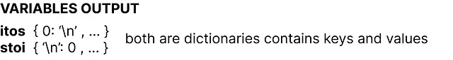
现在,我们正在创建整数到字符的映射(itos)和字符到整数的映射(stoi)。以下是代码:
# Mapping integers to characters (itos)
itos = {i: ch for i, ch in enumerate(vocab)}

# Mapping characters to integers (stoi)
stoi = {ch: i for i, ch in enumerate(vocab)}
在原始的LLaMA论文中,使用了来自Google的SentencePiece字节对编码分词器。然而,为了简化起见,我们将选择一个基本的字符级分词器。让我们创建编码和解码函数,稍后我们将应用于我们的数据集:
# Encode function: Converts a string to a list of integers using the mapping stoi
def encode(s):
    return [stoi[ch] for ch in s]

# Decode function: Converts a list of integers back to a string using the mapping itos
def decode(l):
    return ''.join([itos[i] for i in l])

# Example: Encode the string "hello" and then decode the result
decode(encode("morning"))
最后一行输出的是早晨确认编码和解码功能的正确性。
我们现在将我们的数据集转换为一个torch张量,使用PyTorch来指定其数据类型以进行进一步的操作:
# Convert the dataset into a torch tensor with specified data type (dtype)
dataset = torch.tensor(encode(lines), dtype=torch.int8)

# Display the shape of the resulting tensor
print(dataset.shape)
输出istorch.Size([1115394]) 表明我们的数据集包含约一百一十一万个标记。值得注意的是,这比LLaMA数据集小得多,该数据集包含着一千四百万亿个标记。
我们将创建一个函数负责将数据集分割为训练集、验证集或测试集。在机器学习或深度学习项目中,这些分割对于开发和评估模型非常重要,同样的原则也适用于复制大型语言模型(LLM)的方法。
# Function to get batches for training, validation, or testing
def get_batches(data, split, batch_size, context_window, config=MASTER_CONFIG):
    # Split the dataset into training, validation, and test sets
    train = data[:int(.8 * len(data))]
    val = data[int(.8 * len(data)): int(.9 * len(data))]
    test = data[int(.9 * len(data)):]

    # Determine which split to use
    batch_data = train
    if split == 'val':
        batch_data = val
    if split == 'test':
        batch_data = test

    # Pick random starting points within the data
    ix = torch.randint(0, batch_data.size(0) - context_window - 1, (batch_size,))

    # Create input sequences (x) and corresponding target sequences (y)
    x = torch.stack([batch_data[i:i+context_window] for i in ix]).long()
    y = torch.stack([batch_data[i+1:i+context_window+1] for i in ix]).long()

    return x, y
现在我们已经定义了分割函数,让我们确定两个在这个过程中至关重要的参数:
# Update the MASTER_CONFIG with batch_size and context_window parameters
MASTER_CONFIG.update({
    'batch_size': 8,          # Number of batches to be processed at each random split
    'context_window': 16      # Number of characters in each input (x) and target (y) sequence of each batch
})
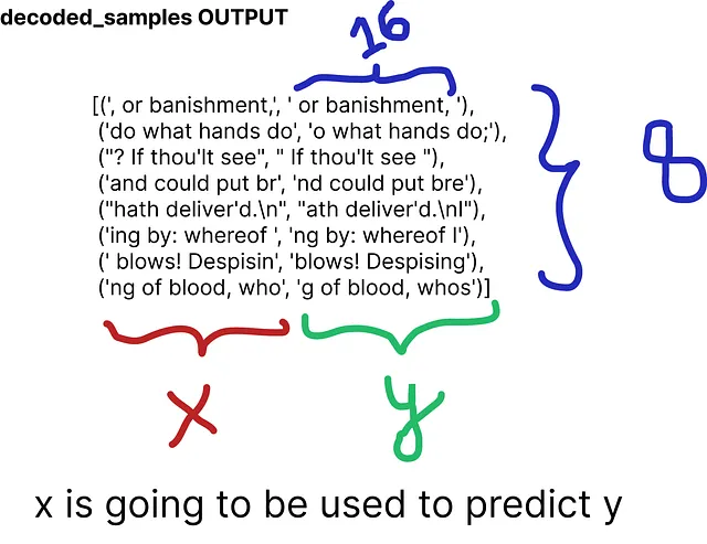
批量大小确定每个随机切分中处理的批次数量,而上下文窗口指定每个批次的输入(x)和目标(y)序列中的字符数量。
让我们从数据集的训练分配和上下文窗口16中打印出批次8的随机样本。
# Obtain batches for training using the specified batch size and context window
xs, ys = get_batches(dataset, 'train', MASTER_CONFIG['batch_size'], MASTER_CONFIG['context_window'])

# Decode the sequences to obtain the corresponding text representations
decoded_samples = [(decode(xs[i].tolist()), decode(ys[i].tolist())) for i in range(len(xs))]

# Print the random sample
print(decoded_samples)
评估策略
现在,我们准备创建一个函数专门用于评估我们自己创建的LLaMA架构。在定义实际的模型方法之前这样做的原因是为了在训练过程中实现持续评估。
@torch.no_grad()  # Don't compute gradients for this function
def evaluate_loss(model, config=MASTER_CONFIG):
    # Placeholder for the evaluation results
    out = {}

    # Set the model to evaluation mode
    model.eval()

    # Iterate through training and validation splits
    for split in ["train", "val"]:
        # Placeholder for individual losses
        losses = []

        # Generate 10 batches for evaluation
        for _ in range(10):
            # Get input sequences (xb) and target sequences (yb)
            xb, yb = get_batches(dataset, split, config['batch_size'], config['context_window'])

            # Perform model inference and calculate the loss
            _, loss = model(xb, yb)

            # Append the loss to the list
            losses.append(loss.item())

        # Calculate the mean loss for the split and store it in the output dictionary
        out[split] = np.mean(losses)

    # Set the model back to training mode
    model.train()

    return out
我们在训练迭代过程中使用损失作为度量模型性能的标准。我们的函数通过训练集和验证集进行迭代,在每个集合上计算10个批次的平均损失,并最终返回结果。然后,使用model.train()将模型重新设置为训练模式。
设置一个基本的神经网络模型
我们正在建立一个基本的神经网络,稍后我们将使用LLaMA技术对其进行改进。
# Definition of a basic neural network class
class SimpleBrokenModel(nn.Module):
    def __init__(self, config=MASTER_CONFIG):
        super().__init__()
        self.config = config

        # Embedding layer to convert character indices to vectors (vocab size: 65)
        self.embedding = nn.Embedding(config['vocab_size'], config['d_model'])

        # Linear layers for modeling relationships between features
        # (to be updated with SwiGLU activation function as in LLaMA)
        self.linear = nn.Sequential(
            nn.Linear(config['d_model'], config['d_model']),
            nn.ReLU(),  # Currently using ReLU, will be replaced with SwiGLU as in LLaMA
            nn.Linear(config['d_model'], config['vocab_size']),
        )

        # Print the total number of model parameters
        print("Model parameters:", sum([m.numel() for m in self.parameters()]))
在目前的架构中,嵌入层的词汇大小为65,表示了我们数据集中的字符。由于这是我们的基准模型,我们在线性层中使用ReLU作为激活函数;然而,后续将用LLaMA中使用的SwiGLU替换它。
为了为我们的基础模型创建一个前向传递(forward pass),我们必须在我们的神经网络模型中定义一个前向函数(forward function)。
# Definition of a basic neural network class
class SimpleBrokenModel(nn.Module):
    def __init__(self, config=MASTER_CONFIG):

        # Rest of the code
        ...

        # Forward pass function for the base model
        def forward(self, idx, targets=None):
            # Embedding layer converts character indices to vectors
            x = self.embedding(idx)

            # Linear layers for modeling relationships between features
            a = self.linear(x)

            # Apply softmax activation to obtain probability distribution
            logits = F.softmax(a, dim=-1)

            # If targets are provided, calculate and return the cross-entropy loss
            if targets is not None:
                # Reshape logits and targets for cross-entropy calculation
                loss = F.cross_entropy(logits.view(-1, self.config['vocab_size']), targets.view(-1))
                return logits, loss

            # If targets are not provided, return the logits
            else:
                return logits

        # Print the total number of model parameters
        print("Model parameters:", sum([m.numel() for m in self.parameters()]))
此前向传递函数以字符索引(idx)作为输入,应用嵌入层,通过线性层传递结果,应用softmax激活函数以获得概率分布(logits)。如果提供目标值,则计算交叉熵损失并返回logits和损失。如果未提供目标值,则仅返回logits。
要实例化这个模型,我们可以直接调用类并打印出我们简单神经网络模型中的参数总数。我们将线性层的维度设置为128,在我们的配置对象中指定这个值。
# Update MASTER_CONFIG with the dimension of linear layers (128)
MASTER_CONFIG.update({
    'd_model': 128,
})

# Instantiate the SimpleBrokenModel using the updated MASTER_CONFIG
model = SimpleBrokenModel(MASTER_CONFIG)

# Print the total number of parameters in the model
print("Total number of parameters in the Simple Neural Network Model:", sum([m.numel() for m in model.parameters()]))

我们的简单神经网络模型包含大约33,000个参数。
同样,为了计算logits和损失,我们只需要将拆分的数据集输入我们的模型中:
# Obtain batches for training using the specified batch size and context window
xs, ys = get_batches(dataset, 'train', MASTER_CONFIG['batch_size'], MASTER_CONFIG['context_window'])

# Calculate logits and loss using the model
logits, loss = model(xs, ys)
为了训练我们的基础模型并记录其性能,我们需要指定一些参数。我们将进行总共1000个周期的训练。将批次大小从8增加到32,并将日志间隔设置为10,这意味着代码将在每10个批次打印或记录有关训练进度的信息。为了优化,我们将使用Adam优化器。
# Update MASTER_CONFIG with training parameters
MASTER_CONFIG.update({
    'epochs': 1000,          # Number of training epochs
    'log_interval': 10,      # Log information every 10 batches during training
    'batch_size': 32,        # Increase batch size to 32
})

# Instantiate the SimpleBrokenModel with updated configuration
model = SimpleBrokenModel(MASTER_CONFIG)

# Define the Adam optimizer for model parameters
optimizer = torch.optim.Adam(
    model.parameters(),      # Pass the model parameters to the optimizer
)
让我们执行训练过程并记录基础模型的损失,包括参数的总数量。此外,为了清晰起见,每一行都有注释。
# Function to perform training
def train(model, optimizer, scheduler=None, config=MASTER_CONFIG, print_logs=False):
    # Placeholder for storing losses
    losses = []

    # Start tracking time
    start_time = time.time()

    # Iterate through epochs
    for epoch in range(config['epochs']):
        # Zero out gradients
        optimizer.zero_grad()

        # Obtain batches for training
        xs, ys = get_batches(dataset, 'train', config['batch_size'], config['context_window'])

        # Forward pass through the model to calculate logits and loss
        logits, loss = model(xs, targets=ys)

        # Backward pass and optimization step
        loss.backward()
        optimizer.step()

        # If a learning rate scheduler is provided, adjust the learning rate
        if scheduler:
            scheduler.step()

        # Log progress every specified interval
        if epoch % config['log_interval'] == 0:
            # Calculate batch time
            batch_time = time.time() - start_time

            # Evaluate loss on validation set
            x = evaluate_loss(model)

            # Store the validation loss
            losses += [x]

            # Print progress logs if specified
            if print_logs:
                print(f"Epoch {epoch} | val loss {x['val']:.3f} | Time {batch_time:.3f} | ETA in seconds {batch_time * (config['epochs'] - epoch)/config['log_interval'] :.3f}")

            # Reset the timer
            start_time = time.time()

            # Print learning rate if a scheduler is provided
            if scheduler:
                print("lr: ", scheduler.get_lr())

    # Print the final validation loss
    print("Validation loss: ", losses[-1]['val'])

    # Plot the training and validation loss curves
    return pd.DataFrame(losses).plot()

# Execute the training process
train(model, optimizer)
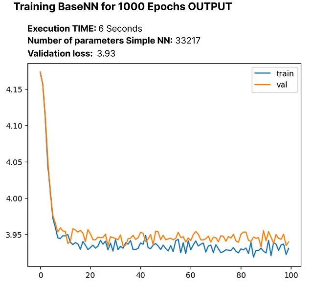
最初训练前的交叉熵损失为4.17,在经过1000个epochs后,降低到3.93。在这个背景中,交叉熵反映了选择错误单词的可能性。
我们的模型在逻辑回归层中加入了softmax层,将一组数字转化为概率分布。让我们使用内置的F.cross_entropy函数,我们需要直接传入未归一化的逻辑回归层输出。因此,我们将相应地修改我们的模型。
# Modified SimpleModel class without softmax layer
class SimpleModel(nn.Module):
    def __init__(self, config):

       # Rest of the code
       ...

    def forward(self, idx, targets=None):
        # Embedding layer converts character indices to vectors
        x = self.embedding(idx)

        # Linear layers for modeling relationships between features
        logits = self.linear(x)

        # If targets are provided, calculate and return the cross-entropy loss
        if targets is not None:

            # Rest of the code
            ...
让我们重新创建更新的SimpleModel,并进行1000个周期的训练以观察任何变化:
# Create the updated SimpleModel
model = SimpleModel(MASTER_CONFIG)

# Obtain batches for training
xs, ys = get_batches(dataset, 'train', MASTER_CONFIG['batch_size'], MASTER_CONFIG['context_window'])

# Calculate logits and loss using the model
logits, loss = model(xs, ys)

# Define the Adam optimizer for model parameters
optimizer = torch.optim.Adam(model.parameters())

# Train the model for 100 epochs
train(model, optimizer)
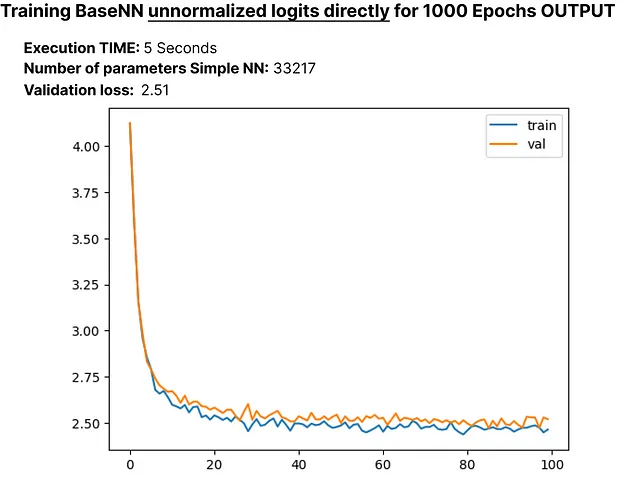
在减少损失为2.51之后,让我们来探索一下我们的语言模型大约有33,000个参数是如何在推理过程中生成文本的。我们将创建一个“generate”函数,在复制LLaMA时稍后会用到。
# Generate function for text generation using the trained model
def generate(model, config=MASTER_CONFIG, max_new_tokens=30):
    idx = torch.zeros(5, 1).long()
    for _ in range(max_new_tokens):
        # Call the model
        logits = model(idx[:, -config['context_window']:])
        last_time_step_logits = logits[
            :, -1, :
        ]  # all the batches (1), last time step, all the logits
        p = F.softmax(last_time_step_logits, dim=-1)  # softmax to get probabilities
        idx_next = torch.multinomial(
            p, num_samples=1
        )  # sample from the distribution to get the next token
        idx = torch.cat([idx, idx_next], dim=-1)  # append to the sequence
    return [decode(x) for x in idx.tolist()]

# Generate text using the trained model
generate(model)
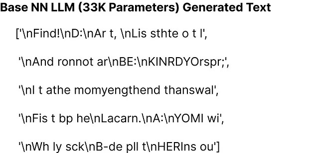
生成的文本不适合我们的基本模型,该模型具有约33K个参数。然而,现在我们已经为这个简单模型奠定了基础,我们将在下一节中开始构建LLaMA架构。
复制LLaMA架构
在博客的前半部分中,我们涵盖了基本概念,现在我们将把这些概念整合到我们的基础模型中。LLaMA对原始Transformer进行了三个架构修改。
- RMSNorm 进行预归一化
- 旋转嵌入
- SwiGLU激活函数
我们将逐个将这些修改融入到我们的基本模型中,并且在此基础上进行迭代和构建。
用于预标准化的RMSNorm
我们正在定义一个具有以下功能的RMSNorm函数:
class RMSNorm(nn.Module):
    def __init__(self, layer_shape, eps=1e-8, bias=False):
        super(RMSNorm, self).__init__()

        # Registering a learnable parameter 'scale' as a parameter of the module
        self.register_parameter("scale", nn.Parameter(torch.ones(layer_shape)))

    def forward(self, x):
        """
        Assumes shape is (batch, seq_len, d_model)
        """
        # Calculating the Frobenius norm, RMS = 1/sqrt(N) * Frobenius norm
        ff_rms = torch.linalg.norm(x, dim=(1,2)) * x[0].numel() ** -.5

        # Normalizing the input tensor 'x' with respect to RMS
        raw = x / ff_rms.unsqueeze(-1).unsqueeze(-1)

        # Scaling the normalized tensor using the learnable parameter 'scale'
        return self.scale[:x.shape[1], :].unsqueeze(0) * raw
我们定义了RMSNorm类。在初始化期间,它注册了一个比例参数。在前向传递过程中,它计算输入张量的Frobenius范数,然后对张量进行归一化。最后,张量被注册的比例参数缩放。这个函数被设计用于在LLaMA中替代LayerNorm操作。
现在是时候将LLaMA的第一个实施概念RMSNorm融合到我们的简单NN模型中了。以下是更新后的代码:
# Define the SimpleModel_RMS with RMSNorm
class SimpleModel_RMS(nn.Module):
    def __init__(self, config):
        super().__init__()
        self.config = config

        # Embedding layer to convert character indices to vectors
        self.embedding = nn.Embedding(config['vocab_size'], config['d_model'])

        # RMSNorm layer for pre-normalization
        self.rms = RMSNorm((config['context_window'], config['d_model']))

        # Linear layers for modeling relationships between features
        self.linear = nn.Sequential(
            # Rest of the code
            ...
        )

        # Print the total number of model parameters
        print("Model parameters:", sum([m.numel() for m in self.parameters()]))

    def forward(self, idx, targets=None):
        # Embedding layer converts character indices to vectors
        x = self.embedding(idx)

        # RMSNorm pre-normalization
        x = self.rms(x)

        # Linear layers for modeling relationships between features
        logits = self.linear(x)

        if targets is not None:

            # Rest of the code
            ...
让我们使用RMSNorm执行修改后的NN模型,并观察模型中更新的参数数量和损失情况:
# Create an instance of SimpleModel_RMS
model = SimpleModel_RMS(MASTER_CONFIG)

# Obtain batches for training
xs, ys = get_batches(dataset, 'train', MASTER_CONFIG['batch_size'], MASTER_CONFIG['context_window'])

# Calculate logits and loss using the model
logits, loss = model(xs, ys)

# Define the Adam optimizer for model parameters
optimizer = torch.optim.Adam(model.parameters())

# Train the model
train(model, optimizer)
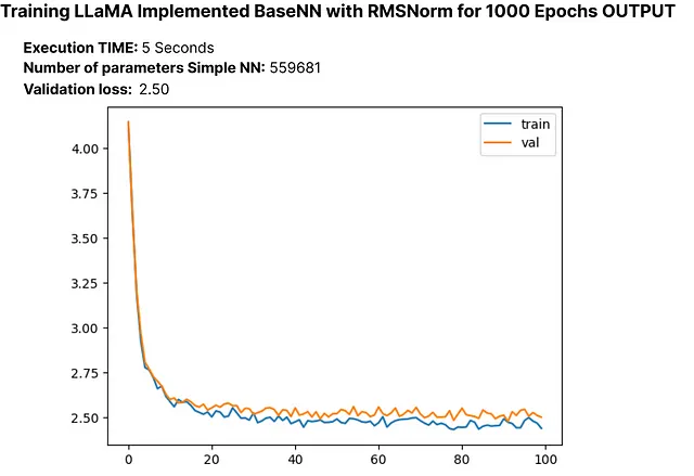
验证损失经历了一个小幅下降,我们更新的LLM参数总数约为55,000个。
旋转嵌入
接下来,我们将实现旋转位置嵌入。在RoPE中,作者建议通过旋转嵌入来嵌入序列中令牌的位置,每个位置应用不同的旋转。让我们创建一个模仿RoPE实际论文实现的函数。
def get_rotary_matrix(context_window, embedding_dim):
    # Initialize a tensor for the rotary matrix with zeros
    R = torch.zeros((context_window, embedding_dim, embedding_dim), requires_grad=False)

    # Loop through each position in the context window
    for position in range(context_window):
        # Loop through each dimension in the embedding
        for i in range(embedding_dim // 2):
            # Calculate the rotation angle (theta) based on the position and embedding dimension
            theta = 10000. ** (-2. * (i - 1) / embedding_dim)
            # Calculate the rotated matrix elements using sine and cosine functions
            m_theta = position * theta
            R[position, 2 * i, 2 * i] = np.cos(m_theta)
            R[position, 2 * i, 2 * i + 1] = -np.sin(m_theta)
            R[position, 2 * i + 1, 2 * i] = np.sin(m_theta)
            R[position, 2 * i + 1, 2 * i + 1] = np.cos(m_theta)
    return R
我们根据指定的上下文窗口和嵌入维度生成一个旋转矩阵,遵循建议的RoPE实现方法。
由于您可能熟悉变压器的架构,其中涉及到注意力头,我们在复制LLaMA时同样需要创建注意力头。首先,让我们使用先前开发用于旋转嵌入的get_rotary_matrix函数创建一个单独的掩码注意力头。另外,每一行都已添加注释以提高清晰度:
class RoPEAttentionHead(nn.Module):
    def __init__(self, config):
        super().__init__()
        self.config = config
        # Linear transformation for query
        self.w_q = nn.Linear(config['d_model'], config['d_model'], bias=False)
        # Linear transformation for key
        self.w_k = nn.Linear(config['d_model'], config['d_model'], bias=False)
        # Linear transformation for value
        self.w_v = nn.Linear(config['d_model'], config['d_model'], bias=False)
        # Obtain rotary matrix for positional embeddings
        self.R = get_rotary_matrix(config['context_window'], config['d_model'])

    def get_rotary_matrix(context_window, embedding_dim):
        # Generate rotational matrix for RoPE
        R = torch.zeros((context_window, embedding_dim, embedding_dim), requires_grad=False)
        for position in range(context_window):
            for i in range(embedding_dim//2):

                # Rest of the code
                ...

        return R

    def forward(self, x, return_attn_weights=False):
        # x: input tensor of shape (batch, sequence length, dimension)

        b, m, d = x.shape  # batch size, sequence length, dimension

        # Linear transformations for Q, K, and V
        q = self.w_q(x)
        k = self.w_k(x)
        v = self.w_v(x)

        # Rotate Q and K using the RoPE matrix
        q_rotated = (torch.bmm(q.transpose(0, 1), self.R[:m])).transpose(0, 1)
        k_rotated = (torch.bmm(k.transpose(0, 1), self.R[:m])).transpose(0, 1)

        # Perform scaled dot-product attention
        activations = F.scaled_dot_product_attention(
            q_rotated, k_rotated, v, dropout_p=0.1, is_causal=True
        )

        if return_attn_weights:
            # Create a causal attention mask
            attn_mask = torch.tril(torch.ones((m, m)), diagonal=0)
            # Calculate attention weights and add causal mask
            attn_weights = torch.bmm(q_rotated, k_rotated.transpose(1, 2)) / np.sqrt(d) + attn_mask
            attn_weights = F.softmax(attn_weights, dim=-1)
            return activations, attn_weights

        return activations
现在我们有了一个返回注意力权重的单个掩码注意力头,下一步是创建一个多头注意力机制。
class RoPEMaskedMultiheadAttention(nn.Module):
    def __init__(self, config):
        super().__init__()
        self.config = config
        # Create a list of RoPEMaskedAttentionHead instances as attention heads
        self.heads = nn.ModuleList([
            RoPEMaskedAttentionHead(config) for _ in range(config['n_heads'])
        ])
        self.linear = nn.Linear(config['n_heads'] * config['d_model'], config['d_model'])  # Linear layer after concatenating heads
        self.dropout = nn.Dropout(.1)  # Dropout layer

    def forward(self, x):
        # x: input tensor of shape (batch, sequence length, dimension)

        # Process each attention head and concatenate the results
        heads = [h(x) for h in self.heads]
        x = torch.cat(heads, dim=-1)

        # Apply linear transformation to the concatenated output
        x = self.linear(x)

        # Apply dropout
        x = self.dropout(x)
        return x
原始论文使用了32个头来实现小得多的7b LLM变体,但由于限制,我们将在我们的方法中使用8个头。
# Update the master configuration with the number of attention heads
MASTER_CONFIG.update({
    'n_heads': 8,
})
现在我们已经实施了旋转嵌入和多头注意力,让我们用更新的代码重新编写我们的RMSNorm神经网络模型。我们将测试其性能,计算损失并检查参数的数量。我们将把这个更新的模型称为“RopeModel”。
class RopeModel(nn.Module):
    def __init__(self, config):
        super().__init__()
        self.config = config

        # Embedding layer for input tokens
        self.embedding = nn.Embedding(config['vocab_size'], config['d_model'])

        # RMSNorm layer for pre-normalization
        self.rms = RMSNorm((config['context_window'], config['d_model']))

        # RoPEMaskedMultiheadAttention layer
        self.rope_attention = RoPEMaskedMultiheadAttention(config)

        # Linear layer followed by ReLU activation
        self.linear = nn.Sequential(
            nn.Linear(config['d_model'], config['d_model']),
            nn.ReLU(),
        )

        # Final linear layer for prediction
        self.last_linear = nn.Linear(config['d_model'], config['vocab_size'])

        print("model params:", sum([m.numel() for m in self.parameters()]))

    def forward(self, idx, targets=None):
        # idx: input indices
        x = self.embedding(idx)

        # One block of attention
        x = self.rms(x)  # RMS pre-normalization
        x = x + self.rope_attention(x)

        x = self.rms(x)  # RMS pre-normalization
        x = x + self.linear(x)

        logits = self.last_linear(x)

        if targets is not None:
            loss = F.cross_entropy(logits.view(-1, self.config['vocab_size']), targets.view(-1))
            return logits, loss

        else:
            return logits
让我们使用RMSNorm、旋转嵌入和掩码多头注意力来执行修改后的NN模型,观察模型中的参数数量以及损失的更新情况。
# Create an instance of RopeModel (RMSNorm, RoPE, Multi-Head)
model = RopeModel(MASTER_CONFIG)

# Obtain batches for training
xs, ys = get_batches(dataset, 'train', MASTER_CONFIG['batch_size'], MASTER_CONFIG['context_window'])

# Calculate logits and loss using the model
logits, loss = model(xs, ys)

# Define the Adam optimizer for model parameters
optimizer = torch.optim.Adam(model.parameters())

# Train the model
train(model, optimizer)
验证损失再次稍微下降,并且我们更新的LLM模型的参数总数大约为55,000。
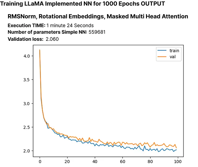
让我们训练模型更多个时期,看看我们重新创建的 LLaMA LLM 的损失是否继续下降。
# Updating training configuration with more epochs and a logging interval
MASTER_CONFIG.update({
    "epochs": 5000,
    "log_interval": 10,
})

# Training the model with the updated configuration
train(model, optimizer)
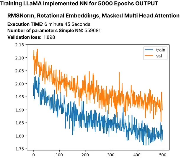
验证损失持续减小,表明训练更多的周期可能会进一步减少损失,尽管不是显著的。
SwiGLU激活函数:
如上所述,LLaMA的创建者使用SwiGLU而不是ReLU,所以我们将在我们的代码中实现SwiGLU方程。

class SwiGLU(nn.Module):
    """ Paper Link -> https://arxiv.org/pdf/2002.05202v1.pdf """
    def __init__(self, size):
        super().__init__()
        self.config = config  # Configuration information
        self.linear_gate = nn.Linear(size, size)  # Linear transformation for the gating mechanism
        self.linear = nn.Linear(size, size)  # Linear transformation for the main branch
        self.beta = torch.randn(1, requires_grad=True)  # Random initialization of the beta parameter

        # Using nn.Parameter for beta to ensure it's recognized as a learnable parameter
        self.beta = nn.Parameter(torch.ones(1))
        self.register_parameter("beta", self.beta)

    def forward(self, x):
        # Swish-Gated Linear Unit computation
        swish_gate = self.linear_gate(x) * torch.sigmoid(self.beta * self.linear_gate(x))
        out = swish_gate * self.linear(x)  # Element-wise multiplication of the gate and main branch
        return out
在Python中实现SwiGLU方程后,我们需要将其集成到我们修改过的LLaMA语言模型(RopeModel)中。
class RopeModel(nn.Module):
    def __init__(self, config):
        super().__init__()
        self.config = config

        # Embedding layer for input tokens
        self.embedding = nn.Embedding(config['vocab_size'], config['d_model'])

        # RMSNorm layer for pre-normalization
        self.rms = RMSNorm((config['context_window'], config['d_model']))

        # Multi-head attention layer with RoPE (Rotary Positional Embeddings)
        self.rope_attention = RoPEMaskedMultiheadAttention(config)

        # Linear layer followed by SwiGLU activation
        self.linear = nn.Sequential(
            nn.Linear(config['d_model'], config['d_model']),
            SwiGLU(config['d_model']),  # Adding SwiGLU activation
        )

        # Output linear layer
        self.last_linear = nn.Linear(config['d_model'], config['vocab_size'])

        # Printing total model parameters
        print("model params:", sum([m.numel() for m in self.parameters()]))

    def forward(self, idx, targets=None):
        x = self.embedding(idx)

        # One block of attention
        x = self.rms(x)  # RMS pre-normalization
        x = x + self.rope_attention(x)

        x = self.rms(x)  # RMS pre-normalization
        x = x + self.linear(x)  # Applying SwiGLU activation

        logits = self.last_linear(x)

        if targets is not None:
            # Calculate cross-entropy loss if targets are provided
            loss = F.cross_entropy(logits.view(-1, self.config['vocab_size']), targets.view(-1))
            return logits, loss

        else:
            return logits
让我们执行带有RMSNorm、旋转嵌入、掩码多头注意力和SwiGLU的修改过的NN模型,以观察模型中更新后的参数数量和损失。
# Create an instance of RopeModel (RMSNorm, RoPE, Multi-Head, SwiGLU)
model = RopeModel(MASTER_CONFIG)

# Obtain batches for training
xs, ys = get_batches(dataset, 'train', MASTER_CONFIG['batch_size'], MASTER_CONFIG['context_window'])

# Calculate logits and loss using the model
logits, loss = model(xs, ys)

# Define the Adam optimizer for model parameters
optimizer = torch.optim.Adam(model.parameters())

# Train the model
train(model, optimizer)
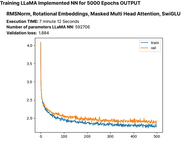
再一次,验证损失经历了小幅下降,并且我们更新的LLM参数现在总计约为60,000。
到目前为止,我们已成功实现了论文的关键组件,即RMSNorm、RoPE和SwiGLU。我们观察到这些实现仅导致损失的轻微降低。
现在我们将为我们的LLaMA添加层来考察它对损失的影响。原始论文在7b版本中使用了32个层,但我们只会使用4个层。让我们相应地调整我们的模型设置。
# Update model configurations for the number of layers
MASTER_CONFIG.update({
    'n_layers': 4,  # Set the number of layers to 4
})
我们先创建一个单一层来了解它的影响。
# add RMSNorm and residual connection
class LlamaBlock(nn.Module):
    def __init__(self, config):
        super().__init__()
        self.config = config

        # RMSNorm layer
        self.rms = RMSNorm((config['context_window'], config['d_model']))

        # RoPE Masked Multihead Attention layer
        self.attention = RoPEMaskedMultiheadAttention(config)

        # Feedforward layer with SwiGLU activation
        self.feedforward = nn.Sequential(
            nn.Linear(config['d_model'], config['d_model']),
            SwiGLU(config['d_model']),
        )

    def forward(self, x):
        # one block of attention
        x = self.rms(x) # RMS pre-normalization
        x = x + self.attention(x)  # residual connection

        x = self.rms(x) # RMS pre-normalization
        x = x + self.feedforward(x)  # residual connection
        return x
创建一个LlamaBlock类的实例并将其应用于一个随机张量。
# Create an instance of the LlamaBlock class with the provided configuration
block = LlamaBlock(MASTER_CONFIG)

# Generate a random tensor with the specified batch size, context window, and model dimension
random_input = torch.randn(MASTER_CONFIG['batch_size'], MASTER_CONFIG['context_window'], MASTER_CONFIG['d_model'])

# Apply the LlamaBlock to the random input tensor
output = block(random_input)
成功创建了一个单层后,我们现在可以使用它来构建多个层。此外,我们将把我们的模型类从“ropemodel”重命名为“Llama”,因为我们已经复制了 LLaMA 语言模型的每个组件。
class Llama(nn.Module):
    def __init__(self, config):
        super().__init__()
        self.config = config
        # Embedding layer for token representations
        self.embeddings = nn.Embedding(config['vocab_size'], config['d_model'])
        # Sequential block of LlamaBlocks based on the specified number of layers
        self.llama_blocks = nn.Sequential(
            OrderedDict([(f"llama_{i}", LlamaBlock(config)) for i in range(config['n_layers'])])
        )
        # Feedforward network (FFN) for final output
        self.ffn = nn.Sequential(
            nn.Linear(config['d_model'], config['d_model']),
            SwiGLU(config['d_model']),
            nn.Linear(config['d_model'], config['vocab_size']),
        )

        # Print total number of parameters in the model
        print("model params:", sum([m.numel() for m in self.parameters()]))

    def forward(self, idx, targets=None):
        # Input token indices are passed through the embedding layer
        x = self.embeddings(idx)
        # Process the input through the LlamaBlocks
        x = self.llama_blocks(x)
        # Pass the processed input through the final FFN for output logits
        logits = self.ffn(x)

        # If targets are not provided, return only the logits
        if targets is None:
            return logits
        # If targets are provided, compute and return the cross-entropy loss
        else:
            loss = F.cross_entropy(logits.view(-1, self.config['vocab_size']), targets.view(-1))
            return logits, loss
让我们使用RMSNorm、旋转嵌入、遮蔽的多头注意力、SwiGLU和N层来执行修改后的LLaMA模型,以观察模型中更新后的参数数量和损失值。
# Create an instance of RopeModel (RMSNorm, RoPE, Multi-Head, SwiGLU, N_layers)
llama = Llama(MASTER_CONFIG)

# Obtain batches for training
xs, ys = get_batches(dataset, 'train', MASTER_CONFIG['batch_size'], MASTER_CONFIG['context_window'])

# Calculate logits and loss using the model
logits, loss = llama(xs, ys)

# Define the Adam optimizer for model parameters
optimizer = torch.optim.Adam(llama.parameters())

# Train the model
train(llama, optimizer)
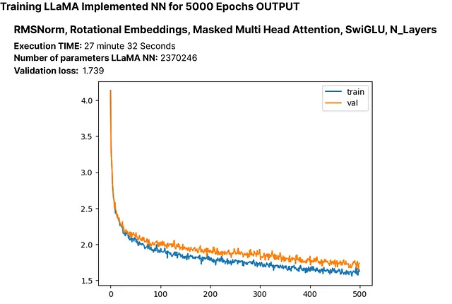
虽然存在过拟合的可能性,但探索增加epochs的数量是否会进一步减少损失非常重要。此外,请注意我们当前的LLM模型具有超过200万个参数。
让我们将其训练更多的轮次。
# Update the number of epochs in the configuration
MASTER_CONFIG.update({
    'epochs': 10000,
})
# Train the LLaMA model for the specified number of epochs
train(llama, optimizer, scheduler=None, config=MASTER_CONFIG)
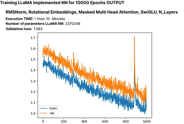
这里的损失为1.08,我们可以在不遇到显著过拟合的情况下实现更低的损失。这表明模型的性能良好。
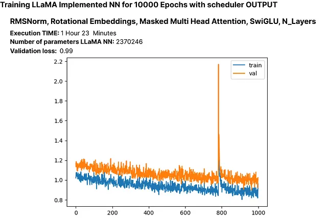
让我们再次训练模型,这次将调度器纳入其中。
# Training the model again, scheduler for better optimization.
train(llama, optimizer, config=MASTER_CONFIG)
到目前为止,我们已经成功地在我们的自定义数据集上实现了LLaMA架构的一个精简版本。现在,让我们来检查从我们的200万参数语言模型生成的输出。
# Generate text using the trained LLM (llama) with a maximum of 500 tokens
generated_text = generate(llama, MASTER_CONFIG, 500)[0]
print(generated_text)
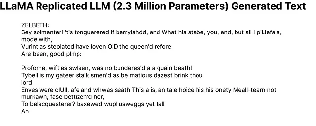
即使有些生成的词语可能不是完美的英语,但我们的带有仅有200万参数的LLM已经展现出对英语的基本理解。
现在,让我们看看我们的模型在测试集上的表现如何。
# Get batches from the test set
xs, ys = get_batches(dataset, 'test', MASTER_CONFIG['batch_size'], MASTER_CONFIG['context_window'])

# Pass the test data through the LLaMA model
logits, loss = llama(xs, ys)

# Print the loss on the test set
print(loss)
在测试集上计算的损失约为1.236。
观察生成输出的变化的简单方法是运行大量的时期进行训练并观察结果。
尝试调整超参数
超参数调整是训练神经网络的关键步骤。在原始的Llama论文中,作者们使用了余弦退火学习率调度。然而,在我们的实验中,它的表现并不好。下面是使用不同学习率调度进行超参数实验的示例:
# Update configuration
MASTER_CONFIG.update({
    "epochs": 1000
})

# Create Llama model with Cosine Annealing learning schedule
llama_with_cosine = Llama(MASTER_CONFIG)

# Define Adam optimizer with specific hyperparameters
llama_optimizer = torch.optim.Adam(
    llama.parameters(),
    betas=(.9, .95),
    weight_decay=.1,
    eps=1e-9,
    lr=1e-3
)

# Define Cosine Annealing learning rate scheduler
scheduler = torch.optim.lr_scheduler.CosineAnnealingLR(llama_optimizer, 300, eta_min=1e-5)

# Train the Llama model with the specified optimizer and scheduler
train(llama_with_cosine, llama_optimizer, scheduler=scheduler)
保存您的语言模型(LLM)
您可以使用以下方法保存您的整个LLM或仅保存参数:
# Save the entire model
torch.save(llama, 'llama_model.pth')

# If you want to save only the model parameters
torch.save(llama.state_dict(), 'llama_model_params.pth')
为了将您的PyTorch模型保存到Hugging Face的Transformers库中,您可以使用save_pretrained方法。以下是一个示例:
from transformers import GPT2LMHeadModel, GPT2Config

# Assuming Llama is your PyTorch model
llama_config = GPT2Config.from_dict(MASTER_CONFIG)
llama_transformers = GPT2LMHeadModel(config=llama_config)
llama_transformers.load_state_dict(llama.state_dict())

# Specify the directory where you want to save the model
output_dir = "llama_model_transformers"

# Save the model and configuration
llama_transformers.save_pretrained(output_dir)
GPT2Config 用于创建与 GPT-2 兼容的配置对象。然后,创建一个 GPT2LMHeadModel 并加载来自 Llama 模型的权重。最后,调用 save_pretrained 来将模型和配置保存到指定目录中。
您可以使用Transformers库加载模型。
from transformers import GPT2LMHeadModel, GPT2Config

# Specify the directory where the model was saved
output_dir = "llama_model_transformers"

# Load the model and configuration
llama_transformers = GPT2LMHeadModel.from_pretrained(output_dir)
结论
在这篇博客中,我们逐步介绍了如何使用LLaMA方法来构建自己的小型语言模型(LLM)的过程。作为建议,考虑将您的模型扩展到约1500万个参数,因为在10M到20M范围内的较小模型往往更能理解英语。一旦您的LLM在语言上表现出色,您可以对其进行特定用途的微调。
我希望这个详尽的博客为您提供了关于复制一篇论文以创建您个人化的硕士法学(LLM)的见解。
感谢阅读这篇长篇文章!